
Engineering blog
September 12, 2026 Michael Freeman
Anatomy of an Anomaly Episode
How the agent scores every metric series it collects, what opens and closes an episode, where the hour-of-week baselines come from, why a bursty interface stays quiet, and how capacity runway is decided, walked through with findings from one Saturday on our lab network.
Every metric the ServiceRadar agent collects is scored where it is collected. An interface counter polled over SNMP, a CPU gauge from the host sampler, the used percentage of a mounted filesystem: each one is a series, and each series gets its own small detector that runs on the agent and never waits for a round trip to the server. The server hears from a detector when it opens an episode, while one is open, and when it closes one. This post is about what that detector does, what it publishes when it fires, and how the same idea extends to the slower questions: is this hour unusual for a Tuesday, and when does this disk fill up.
Four signals per series
The detector lives in the anomaly add-on, a Rust process the agent runs beside its
collectors. The statistics are ours, in the
serviceradar-anomaly-core
crate: a Welford accumulator for the running summary, a median and MAD estimator for
the robust scale, the CUSUM, the seasonal buckets, and an ESD and robust-PCA pair
used offline for scoring. What we take from
DeepCausality
is the frame those statistics run in, and it is worth being precise about that,
because the name suggests causal inference and there is none here. Two of its crates
are in use. The sliding window that holds a series' recent samples is DeepCausality's
window type over a vector store, which gives a fixed-capacity, append-only view with
the arithmetic already correct for the wraparound. And the detector itself is written
as a CausalFlow: a typed pipeline where each stage receives the window state, the
thresholds, and a value, and hands the next stage a new one. The flow hydrates the
window, evaluates the signals, branches on whether the sample breached (a breaching
sample is admitted to the window bounded to the pre-sample decision interval, so a
sustained regime keeps aging the window without teaching it that the regime is
normal; a clean sample is admitted as is), and finalizes a verdict. The point of
writing it that way is that every stage is a function of explicit inputs with no
hidden state, so the same code runs on the agent, in the offline scoring harness, and
in a test that feeds it one sample at a time and inspects the verdict. Nothing in it
builds a causal model, intervenes, or asks counterfactual questions.
For each series the flow evaluates four signals against every new value.
The first is a rolling z-score over the last 300 samples. It uses the median and the median absolute deviation rather than the mean and standard deviation, so a single extreme sample moves the baseline very little and one spike cannot make the next spike look normal. A value more than three MADs from the median breaches. The second is the same z-score computed against a seasonal baseline: not the last 300 samples, but the values this series has produced at this hour on this weekday over the last several weeks. The baseline is built on the server from the hourly rollups, 168 buckets per series, and shipped to the agent with its add-on configuration. A bucket only counts once it holds at least four samples, and each week contributes one, so a series needs about a month of history before its seasonal view switches on. The third signal is a CUSUM, a cumulative sum of deviations that catches a slow drift the z-scores are blind to, because a change of half a MAD per hour never trips a threshold of three but adds up. The fourth is a burst envelope, and it deserves its own section.
A signal breaches on one slot; an episode needs consecutive breaching slots, one by default and configurable per metric class. When the confirmation count is met the detector opens an episode, and it keeps the episode open until every signal that is ready reports clean again. Then it closes it with a reason. Each transition is published as an OCSF finding over the agent's normal record path, and the finding carries the evidence the decision was made on. This is the clear event for an interface on one of our lab switches, trimmed:
{
  "state": "anomaly_clear",
  "value": 37037.88,
  "reason": "all ready signals are clean; consecutive anomalous slots reset",
  "signals": [
    {"name": "rolling",  "mean": 39374.17, "stddev": 4122.93, "score": 0.07,
     "reason": "rolling z-score 0.071 is below 3.000", "sample_count": 300},
    {"name": "seasonal", "mean": 19849.87, "stddev": 1115.85, "score": 0.52,
     "reason": "seasonal z-score 0.525 is below 3.000", "sample_count": 32}
  ],
  "episode_peak_value": 1108392.05,
  "clear_reason": "recovered",
  "producer_version": "0.3.7"
}
Everything needed to argue with the detector is in there. The port normally moves about 39 KB/s with a spread of 4 KB/s. It peaked at 1.1 MB/s during the episode. The current value is 37 KB/s, which is 0.07 MADs from the rolling median and half a MAD from what this hour of the week usually looks like. Both views agree it is over. The server stores the episode keyed by series, folds any duplicate delivery of the same transition into the existing row, and the device page shows the episode with the same numbers.
What an episode looks like
The switch in the payload above is
aruba-24g-02
, an access switch in the lab. At 12:43 UTC on a Saturday, port 23 went from
40 KB/s to 1.1 MB/s outbound and stayed there for five minutes. Inbound and outbound
octets and packets all breached in the same minute, so four episodes opened, one per
counter.
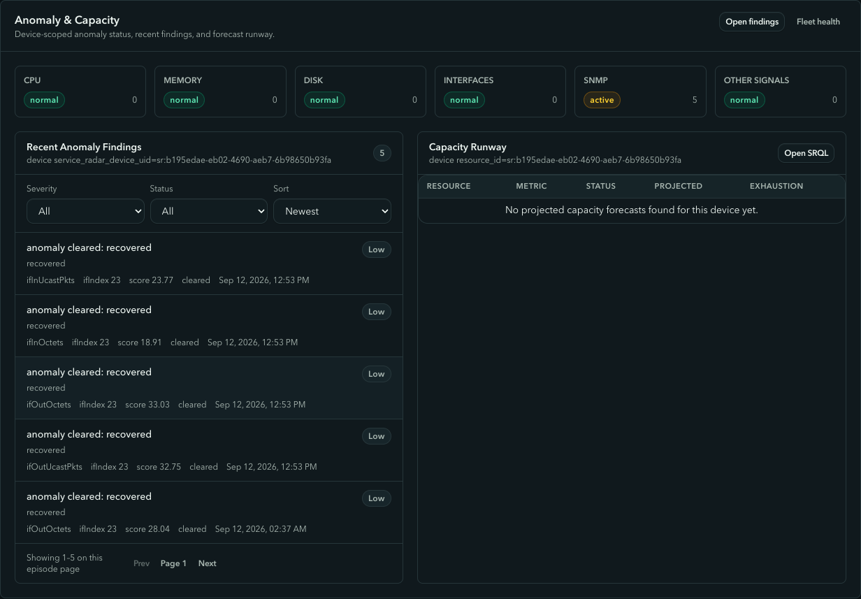
Opening one of them shows the metric context the detector had: the interface's own outbound rate over the surrounding hours, with the finding window marked.
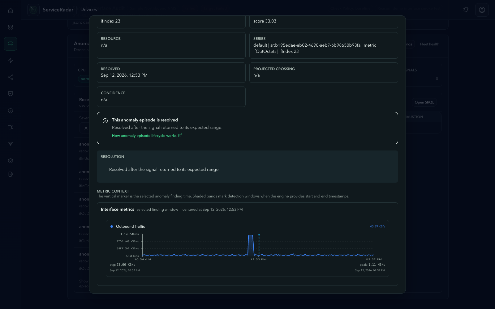
The episodes cleared at 12:53, when the rate had been back at its baseline for long enough that the rolling score dropped under three. The raw counter tells the same story without the detector: about 66 MB per minute for five minutes, 2 to 4 MB per minute before and after. The same port did the same thing at 02:26 that morning, so something behind it moves a few hundred megabytes twice a day. Whether that matters is a question for the person who owns the port; the detector's job is to make the answer cheap to reach.
The burst envelope
The lab's edge router,
tonka01
, has an interface that carries a burst of several hundred KB/s for a few
minutes every twenty minutes, on a link whose rolling median sits near 14 KB/s. A
z-score sees a fifty-sigma event three times an hour, forever. The score is correct,
since the value really is fifty MADs from the median, and it is useless. The seasonal
baseline does not help either, because at a one-hour bucket size the burst averages into
the rest of the hour.
The burst envelope is the fourth signal, and it exists for exactly this series. It keeps a tail of the series' own recent raw values, lagged behind the present, and computes an envelope from a high quantile of that tail times a multiplier. A sample inside the envelope is a burst this series has already shown it produces, and it does not count as a breach even when the other signals fire. The one subtlety is that the tail is frozen at the moment a breaching run starts. Without that, a surge that lasts a few minutes would feed itself into the envelope, the envelope would grow to cover it, and the episode would close as recovered while the surge was still going. With it, a burst that matches the interface's history is quiet and a burst that does not is an episode.
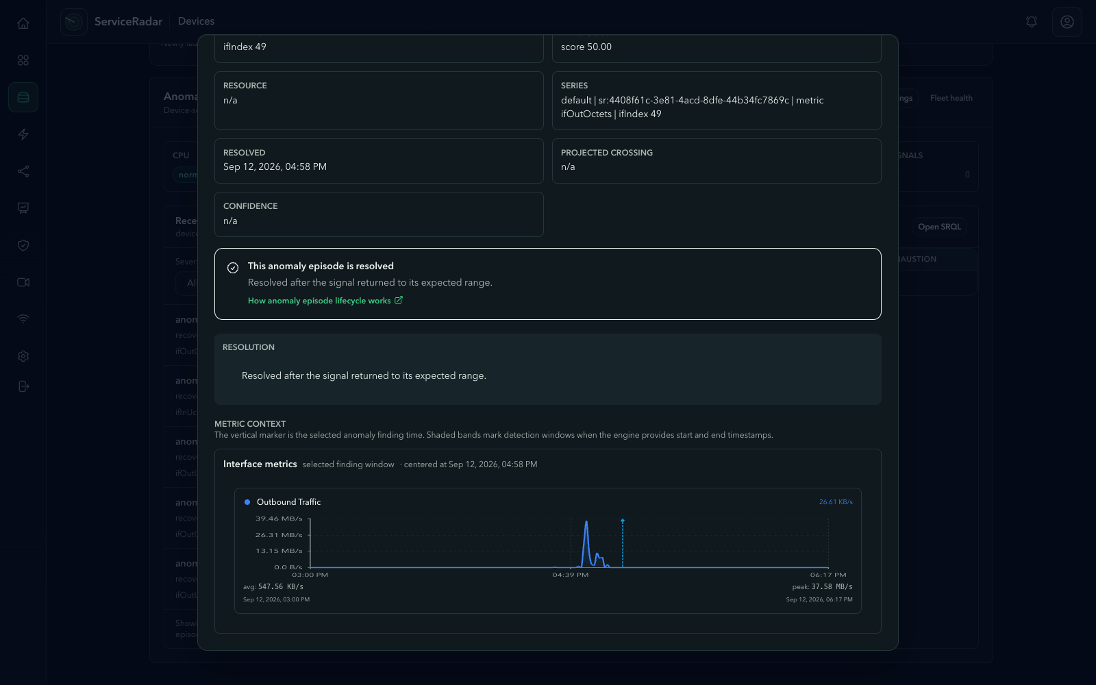
The same router showed the difference that Saturday. At 16:44 UTC it pushed about 2 GB per minute out of two interfaces for eight minutes, roughly 37 MB/s on links that idle at tens of kilobytes. Five episodes opened across the three interfaces involved and all five cleared by 17:03 when the transfer ended. The twenty-minute interface produced nothing, because nothing about it changed.
Where the hour-of-week baselines come from
The agent cannot build a seasonal baseline on its own; it would need weeks of history it does not keep. The server does. Once an hour a producer job walks every device that has an anomaly add-on, reads the hourly rollups for each of its series over the baseline window, and computes a median and MAD for every one of the 168 weekday-hour buckets. It does this one device at a time, because a single query across a whole fleet of hosts runs longer than the database's statement timeout, and it records a health heartbeat with the count of series it delivered and the sources it could not. The baselines ride to the agent inside the add-on assignment, the same channel that carries the detector's thresholds, so a change to either arrives the same way.
Host gauges like CPU and memory get a second seasonal pass on the server itself. A worker runs at 47 minutes past each hour, takes the hourly average that just completed for each series, and scores it against the same weekday-hour bucket with the same median-and-MAD arithmetic. Its verdicts carry the evaluation time, the bucket it judged and a one-sentence reason, and they open and close episodes exactly as the agent's do. This is the pass that catches the thing a z-score on live samples cannot: an hour that is unremarkable on its own and wrong for when it happened.
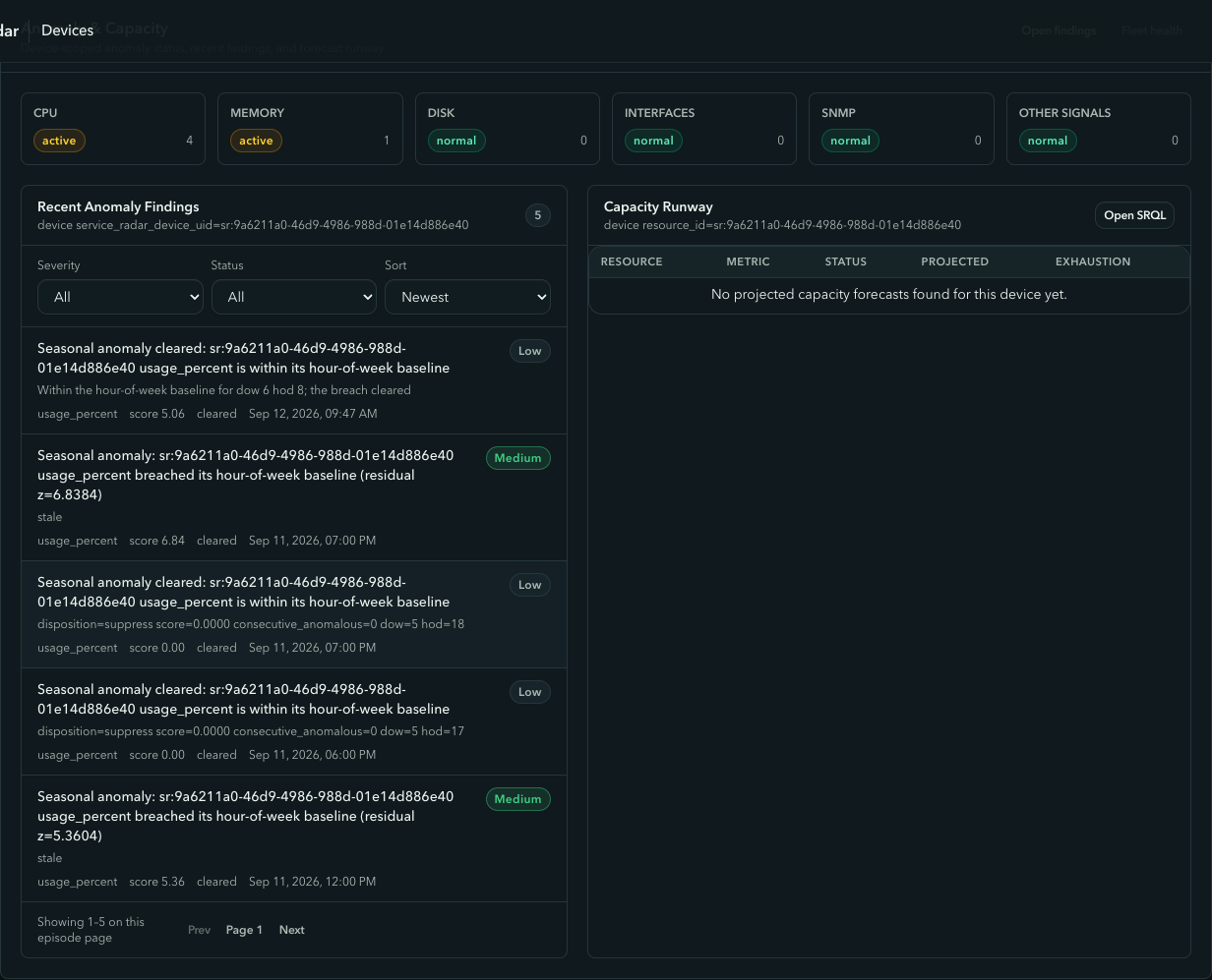
k8s-cp3-worker1
is a Kubernetes node in the lab. Its 07:00 UTC hour runs a job that takes CPU to
between 70 and 100 percent on most days, and had done so on every Saturday in the
baseline window. On this Saturday the hour peaked at 5 percent.
| Day | Weekday | Avg CPU, 07:00 UTC | Peak CPU, 07:00 UTC |
|---|---|---|---|
| 2026-09-05 | Sat | 26.0 % | 100.0 % |
| 2026-09-06 | Sun | 13.2 % | 74.9 % |
| 2026-09-07 | Mon | 11.2 % | 56.3 % |
| 2026-09-08 | Tue | 2.5 % | 31.3 % |
| 2026-09-09 | Wed | 5.0 % | 99.9 % |
| 2026-09-11 | Fri | 10.2 % | 95.9 % |
| 2026-09-12 | Sat | 1.5 % | 5.1 % |
Nothing spiked. The hour was quiet, and quiet is the anomaly. The seasonal worker opened an episode at 08:47 with a score of 5.06 against the Saturday 07:00 bucket, and closed it an hour later when 08:00 matched its own bucket. Absent load is one of the more useful things a monitor can notice, and one of the hardest to write a static threshold for, because the threshold would have to know what day it is.
Alerts follow episodes
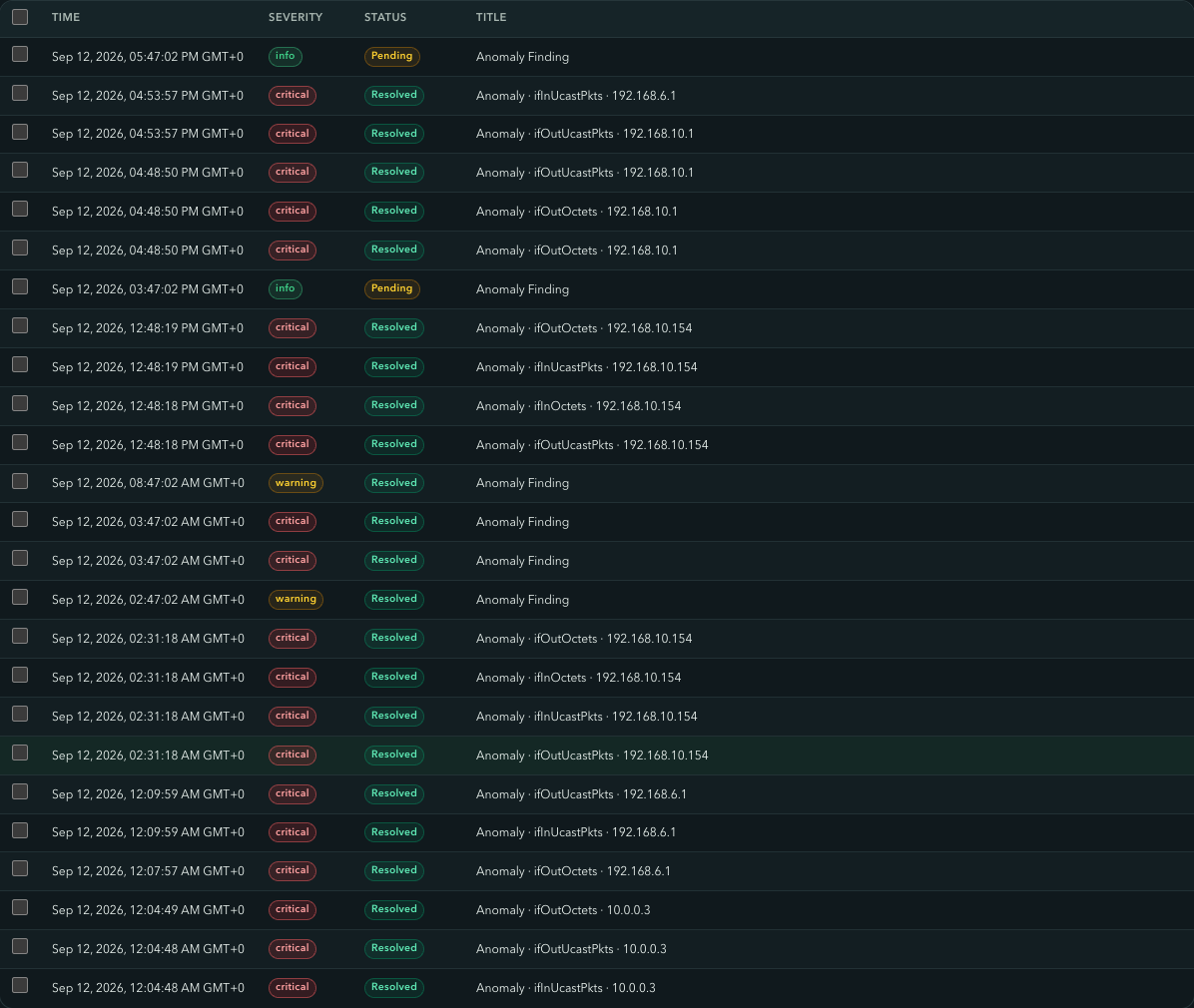
An alert is a view of an episode, not a separate judgement. A seeded rule turns the open transition into an alert and the clear transition into its resolution, grouped by the series, so nobody closes anomaly alerts by hand. On the Saturday above the fleet raised a dozen across three devices, and every one whose episode cleared resolved itself within fifteen minutes.
The pipeline watches itself the same way. The baseline producer, the seasonal worker and the capacity forecaster each record a health check when they run, and a rule promotes a check going unhealthy into a critical alert. A detector that silently stops receiving baselines is the failure mode that is easiest to miss, because the symptom is fewer findings, and fewer findings looks like a quiet network.
Capacity runway, and why the table is usually empty
Capacity forecasting is the slow cousin of the detector. Once an hour it takes each consumable resource, disk usage per mount and memory usage per host by default, fits a trend to its hourly history and projects when the trend crosses the resource's threshold. It reports a runway only when the projection is worth reporting, and that takes four things: enough history for the model, a slope whose confidence interval excludes zero, a lower prediction bound that still reaches the threshold at the horizon, and a crossing no further out than twice the history it was fitted on. A trend with three days behind it can project a crossing in 2031; the last gate is what keeps 2031 off the table.
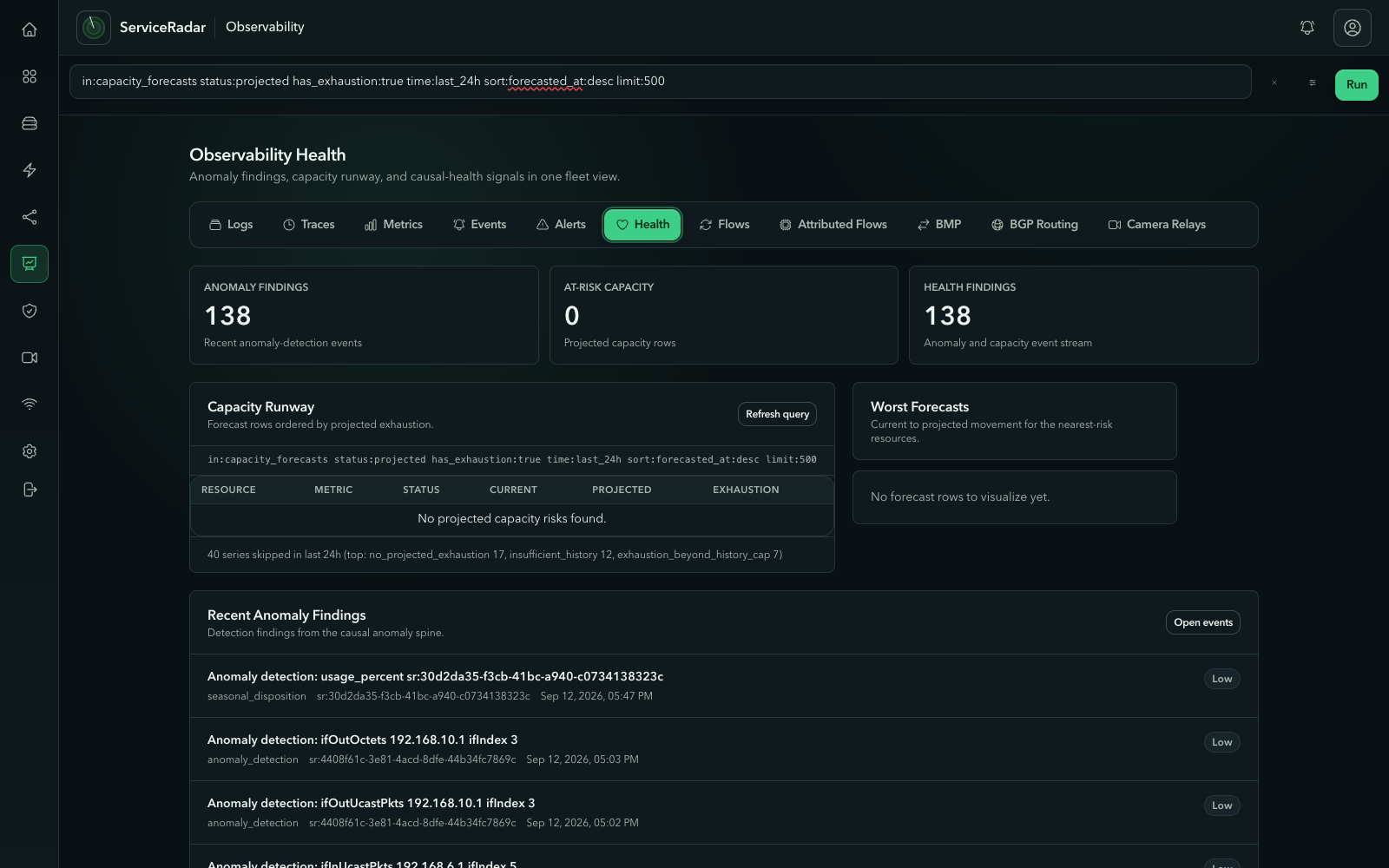
On the lab fleet that Saturday the forecaster looked at 40 series and put none on the
runway table, which is the right answer. Seventeen have no upward trend. Twelve have
less than a day of history. Four are flat. Seven are growing, but six of them cross
their threshold in 2027 or later and the seventh, a checker volume growing about half a
point a day, crosses 80 percent in November with 25 days of history behind it. It is
recorded as
exhaustion_beyond_history_cap
with the projected date, and it moves onto the table by itself once its history covers
half the distance to the crossing. Every skipped series is counted by reason in the line
under the table, so an empty table and a dead forecaster do not look alike.
Looking for yourself
All of this is ordinary data in the same database the UI reads, and SRQL reaches all of it. The findings stream, the hourly rollups the baselines are built from, the per-mount disk rollup and the forecast rows are a query each:
in:events event_type:(anomaly,anomaly_detection) time:last_24h sort:time:desc limit:50
in:timeseries_metric_interface_hourly device_id:"<device uid>" if_index:23 time:last_7d sort:bucket:asc
in:timeseries_metric_disk_hourly metric_name:"disk.used_percent" device_id:"<device uid>" time:last_30d
in:capacity_forecasts time:last_24h sort:forecasted_at:desc limit:100
The signals, thresholds and per-class overrides are documented in Anomaly Detection and the Anomaly Engine reference, and the detector itself is rust/anomaly-core in the main repository.